Wojtek Sterna

If you want to be notified about future posts, please consider subscribing:

In 3D graphics a typical perspective projection matrix takes, as one of its arguments, the vertical field of view. As an example have a look at DirectX’s D3DXMatrixPerspectiveFovLH function.

In video games, quite often the wider the aspect ratio of the rendering resolution, the wider the horizontal field of view [1]. Some games (first person games) often go as far as to allow players to configure field of view to their liking. So it turns out that in practice we more often than not need to work with the horizontal field of view, and not the vertical field of view that most perspective matrix math is based on. As such, it is convenient to have functions with which we can convert vertical field of view to horizontal and vice versa.

At first I thought these formulas would be easy. I thought that to convert from the vertical field of view to horizontal all we need to do is to multiply the vertical field of view by the screen’s aspect ratio. It’s a little bit more complicated than that.

1. Math Formulas

Let’s go straight into the formulas for conversion. Derivation of those formulas is presented in the next section.

On input we need the screen’s aspect ratio $A$ .
We also denote the vertical field of view as $V$ and horizontal field of view as $H$ .

Now, given the vertical field of view $V$ the formula for horizontal field of view $H$ is:

$H = 2 \cdot \tan^{-1} \left( A \cdot \tan \left( \cfrac{V}{2} \right) \right)$

The opposite, given the horizontal field of view $H$ the formula for vertical field of view $V$ is:

$V = 2 \cdot \tan^{-1} \left( \cfrac{1}{A} \cdot \tan \left( \cfrac{H}{2} \right) \right)$

2. Derivation of the Formulas

Derivation of the formulas we start off with an illustration of the view frustum:

The view frustum has the tip, which is the point where the camera/eye is located. Distance $n$ away is the near plane, and distance $f$ away is the far plane. Typically all triangles that are within the frustum’s bounds (the grey area) are projected onto the near plane and that is what ends up being displayed to the viewer.

Let’s now have a look at the side section of the frustum:

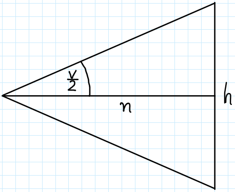
What we are seeing in this image is only the part from the eye to the near plane — to the left there is the eye and to the right, next to letter “h” is the near plane. Actually, the letter “h” denotes the near plane’s height $h$ .
Other variables in this image are the distance to the near plane $n$ and half of the vertical field of view’s angle $\cfrac{V}{2}$ .
We can tie all these variables together with the following equation:

$\tan \left( \cfrac{V}{2} \right) = \cfrac{0.5 \cdot h}{n}$

Now let’s have a look at the frustum’s top section (birdseye view):

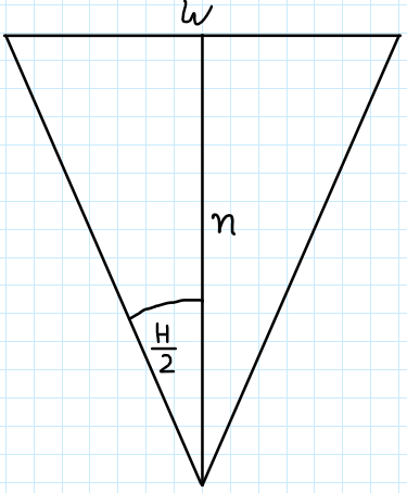
This one is similar but now instead of the height we have the near plane’s width $w$ and instead of the vertical field of view’s half-angle we have the horizontal’s $\cfrac{H}{2}$ .
Equation that ties all these variables is:

$\tan \left( \cfrac{H}{2} \right) = \cfrac{0.5 \cdot w}{n}$

We now have two equations that both sport the same variable $n$ in them. Slight manipulation of these equations leads to:

$n = \cfrac{0.5 \cdot h}{\tan \left( \cfrac{V}{2} \right)}$

$n = \cfrac{0.5 \cdot w}{\tan \left( \cfrac{H}{2} \right)}$

We can now write:

$\cfrac{0.5 \cdot h}{\tan \left( \cfrac{V}{2} \right)} \quad = \quad \cfrac{0.5 \cdot w}{\tan \left( \cfrac{H}{2} \right)}$

This equation ties together the vertical field of view $V$ and horizontal field of view $H$ . Assuming we know the near plane’s width $w$ and height $h$ we can now easily calculate $H$ as a function of $V$ (and vice versa):

$H = 2 \cdot \tan^{-1} \left( \cfrac{w}{h} \cdot \tan \left( \cfrac{V}{2} \right) \right)$

This formula requires us to know the near plane’s width $w$ and height $h$ . Note though that we actually only need the ratio of those values, not the values themselves, and that ratio will be constant throughout the entire view frustum (and beyond). So we don’t actually need the exact near plane size, we only need the ratio $A$ which we can calculate from the application window’s width and height for example. This leads us to the final formula:

$H = 2 \cdot \tan^{-1} \left( A \cdot \tan \left( \cfrac{V}{2} \right) \right)$

Derivation of the formula for $V$ follows the same pattern.

3. Example Application

On GitHub you can find an example application demonstrating the above formula in action.

Here’s C# source code implementing the formulas:

private float MyVerticalToHorizontalFieldOfView(float fovY, float aspect)
{
	fovY *= Mathf.Deg2Rad;
	float fovX = 2.0f * Mathf.Atan(aspect * Mathf.Tan(fovY / 2.0f));
	return fovX * Mathf.Rad2Deg;
}

private float MyHorizontalToVerticalFieldOfView(float fovX, float aspect)
{
	fovX *= Mathf.Deg2Rad;
	float fovY = 2.0f * Mathf.Atan(1.0f/aspect * Mathf.Tan(fovX / 2.0f));
	return fovY * Mathf.Rad2Deg;
}

The functions above assume that the vertical and horizontal field of views, fovX and fovY are given in degrees and that the output values are also in degrees. Functions Mathf.Tan and Mathf.Atan oparate in radians hence the need for a few conversions.

In function Update of the Unity script we have:

void Update()
{
	float aspect = (float)Screen.width / (float)Screen.height;
	float fovY = Camera.main.fieldOfView;
	float fovX;

	fovX = Camera.VerticalToHorizontalFieldOfView(fovY, aspect);
	fovY = Camera.HorizontalToVerticalFieldOfView(fovX, aspect);
	Debug.Log("Unity's:    " + fovY + "    " + fovX);

	fovX = MyVerticalToHorizontalFieldOfView(fovY, aspect);
	fovY = MyHorizontalToVerticalFieldOfView(fovX, aspect);
	Debug.Log("My:    " + fovY + "    " + fovX);
}

In this code we first read the camera’s (vertical) field of view and calculate the aspect ratio. Then, we convert the vertical fov (field of view) to horizontal and then back to vertical (we should end up with the same value we started with).
The conversion is carried out using two different sets of functions — first with Unity’s built-in functions and then with our implementations. This way we can confirm that our implementations work correctly.

4. Bibliography

[1] Field of view in video games, https://en.wikipedia.org/wiki/Field_of_view_in_video_games

Vertex Projection onto a Plane

25 May 202310 January 2024Wojtek SternaLeave a comment

View all posts

If you want to be notified about future posts, please consider subscribing:

This blog post is a “port” into native website form of a LaTeX/PDF article that I wrote back in 2008, named Vertex Projection onto a Plane. Motivation for that was to play with LaTeX in WordPress. I have not introduced any corrections.

Projection is important graphics operation. We use projection to make our 3-dimensional world appear on a 2-dimensional screen, we use dot product to project one vector onto another. In this article we will derive matrices that project a vertex onto a plane.

If you still do not know what it is for I will give you a brief example. Imagine you want your object to cast a shadow onto a ground plane. You could achieve this by projecting all object’s vertices onto that plane. What you get is your object flattened on the plane just as it would cast a shadow. Such object could be projected from a specific direction (a directional light generating shadows) or from a specific point (a point light generating shadows). We will consider both cases.

1. Directional Projection

Let’s start with some formulas:

$x = x_0 + at$

$y = y_0 + bt$

$z = z_0 + ct$

$Ax + By + Cz + D = 0$

What we have here is the straight line equation with projection direction $[a, b, c]$ , vertex $(x_0, y_0, z_0)$ we are projecting and the plane equation $[A, B, C, D]$ we are projecting onto. Our main task is to find $t$ .

To find $t$ we need to substitute $x$ , $y$ and $z$ equations to the plane equation and solve for $t$ . In other words we want to find such $t$ for which a point on our straight line also lies on the plane. We have:

$Ax + By + Cz + D = 0$

$A(x_0 + at) + B(y_0 + bt) + C(z_0 + ct) + D = 0$

$Ax_0 + Aat + By_0 + Bbt + Cz_0 + Cct + D = 0$

$t(Aa + Bb + Cc) = -(Ax_0 + By_0 + Cz_0 + D)$

$t = - \cfrac{Ax_0 + By_0 + Cz_0 + D}{Aa + Bb + Cc}$

At this point we actually have the solution we were looking for. If we substitute this just calculated $t$ value to our initial straight line equation we will have a position $(x, y, z)$ of vertex $(x_0, y_0, z_0)$ projected onto a plane $[A, B, C, D]$ along $[a, b, c]$ direction.

Although we have a proper solution it would be much better to have it in a matrix form. Such a matrix form is convenient, for example, when we use vertex shaders. What we do is just passing the computed matrix to a shader and letting it do the projection in a fast GPU way.

To derive the projection matrix we need to solve $x$ , $y$ and $z$ equations with substituting $t$ and rearrange them a bit. Let’s first solve $x$ for $t$ :

$x = x_0 + at$

$x = x_0 - a\cfrac{Ax_0 + By_0 + Cz_0 + D}{Aa + Bb + Cc}$

$x = x_0 - \cfrac{aAx_0}{Aa + Bb + Cc}$ $- \cfrac{aBy_0}{Aa + Bb + Cc}$ $- \cfrac{aCz_0}{Aa + Bb + Cc}$ $- \cfrac{aD}{Aa + Bb + Cc}$

$x = x_0(1 - \cfrac{aA}{Aa + Bb + Cc})$ $+ y_0(- \cfrac{aB}{Aa + Bb + Cc})$ $+ z_0(- \cfrac{aC}{Aa + Bb + Cc})$ $+ (- \cfrac{aD}{Aa + Bb + Cc})$

Solving $y$ and $z$ for $t$ in the same way yields:

$y = x_0(- \cfrac{bA}{Aa + Bb + Cc})$ $+ y_0(1 - \cfrac{bB}{Aa + Bb + Cc})$ $+ z_0(- \cfrac{bC}{Aa + Bb + Cc})$ $+ (- \cfrac{bD}{Aa + Bb + Cc})$

$z = x_0(- \cfrac{cA}{Aa + Bb + Cc})$ $+ y_0(- \cfrac{cB}{Aa + Bb + Cc})$ $+ z_0(1 - \cfrac{cC}{Aa + Bb + Cc})$ $+ (- \cfrac{cD}{Aa + Bb + Cc})$

Now let’s introduce a helper variable $k$ such that:

$k = -\cfrac{1}{Aa + Bb + Cc}$

Now:

$x = x_0(1 + kaA) + y_0(kaB) + z_0(kaC) + kaD$

$y = x_0(kbA) + y_0(1 + kbB) + z_0(kbC) + kbD$

$z = x_0(kcA) + y_0(kcB) + z_0(1 + kcC) + kcD$

You may not see it yet but we have just derived our matrix form! Take a look:

$\begin{bmatrix} x & y & z & w \end{bmatrix} = \begin{bmatrix} x_0 & y_0 & z_0 & 1 \end{bmatrix} \begin{bmatrix} 1 + kaA & kbA & kcA & 0 \cr kaB & 1 + kbB & kcB & 0 \cr kaC & kbC & 1 + kcC & 0 \cr kaD & kbD & kcD & 1 \end{bmatrix}$

And that’s it. Our projection matrix has been derived. Note that the 4th column is made of $[0, 0, 0, 1]$ vector. That means this matrix doesn’t do any perspective transformation so we may be sure that $w$ will always be equal to 1. Dividing $x$ , $y$ and $z$ by $w$ is not necessary.

2. Point Projection

Point projection is very similar to directional. The only thing that is different is that the projection vector is unique for every object’s vertex $(x_0, y_0, z_0)$ and depends on projector’s (point) position $(d, e, f)$ . Initial formulas:

$x = d + (x_0 - d)t$

$y = e + (y_0 - e)t$

$z = f + (z_0 - f)t$

$Ax + By + Cz + D = 0$

So as you can see, the equations are very similar to those used in directional projection. The only change is that we consider projector’s position.

Just as in direction projection we must first find $t$ by substituting $x$ , $y$ and $z$ to the plane equation:

$Ax + By + Cz + D = 0$

$A(d + (x_0 - d)t) + B(e + (y_0 - e)t) + C(f + (z_0 - f)t) + D = 0$

$(Ad + Ax_0t - Adt) + (Be + By_0t - Bet) + (Cf + Cz_0t - Cft) + D = 0$

$t(Ax_0 - Ad + By_0 - Be + Cz_0 - Cf) = -(Ad + Be + Cf + D)$

$t = -\cfrac{Ad + Be + Cf + D}{Ax_0 - Ad + By_0 - Be + Cz_0 - Cf}$

Solving $x$ for $t$ yields:

$x = d + (x_0 - d)t$

$x = d - \cfrac{(x_0 - d)(Ad + Be + Cf + D)}{Ax_0 + By_0 + Cz_0 - (Ad + Be + Cf)}$

$x = \cfrac{d(Ax_0 + By_0 + Cz_0 - (Ad + Be + Cf))}{Ax_0 + By_0 + Cz_0 - (Ad + Be + Cf)}$ $- \cfrac{(x_0 - d)(Ad + Be + Cf + D)}{Ax_0 + By_0 + Cz_0 - (Ad + Be + Cf)}$

$x = \cfrac{d(Ax_0 + By_0 + Cz_0) - d(Ad + Be + Cf) - x_0(Ad + Be + Cf + D) + d(Ad + Be + Cf) + dD}{Ax_0 + By_0 + Cz_0 - (Ad + Be + Cf)}$

$x = \cfrac{dAx_0 + dBy_0 + dCz_0 - x_0Ad - x_0Be - x_0Cf - x_0D + dD}{Ax_0 + By_0 + Cz_0 - (Ad + Be + Cf)}$

$x = \cfrac{x_0(-Be - Cf - D) + y_0(dB) + z_0(dC) + dD}{Ax_0 + By_0 + Cz_0 - (Ad + Be + Cf)}$

Solving $y$ and $z$ for $t$ in the same way yields:

$y = \cfrac{x_0(eA) + y_0(-Ad - Cf - D) + z_0(eC) + eD}{Ax_0 + By_0 + Cz_0 - (Ad + Be + Cf)}$

$z = \cfrac{x_0(fA) + y_0(fB) + z_0(-Ad - Be - D) + fD}{Ax_0 + By_0 + Cz_0 - (Ad + Be + Cf)}$

And so we have – the matrix form is now easy to be written down. You may be worried about the denominator, as vertex $(x_0, y_0, z_0)$ appears there, so you may think it is not correct. If so you probably forgot about one – perspective division. Dividing by $w$ will be necessary here. The final matrix:

$\begin{bmatrix} x & y & z & w \end{bmatrix} = \begin{bmatrix} x_0 & y_0 & z_0 & 1 \end{bmatrix} \begin{bmatrix} -(Be + Cf + D) & eA & fA & A \cr dB & -(Ad + Cf + D) & fB & B \cr dC & eC & -(Ad + Be + D) & C \cr dD & eD & fD & -(Ad + Be + Cf) \end{bmatrix}$

After transformation all you have left is to divide $x$ , $y$ and $z$ by $w$ .

3. Acknowledgments

I would like to thank to Krzysztof Kluczek for helping me in developing these formulas (via gamedev.pl forum).

Quaternions and Gimbal Lock (Unity 3D)

23 May 202315 November 2025Wojtek SternaLeave a comment

View all posts

If you want to be notified about future posts, please consider subscribing:

Quaternions do not solve the gimbal lock problem. There. I said it in bold font to confirm your suspicion :). I guess you’ve read in many places something along the lines of:
“Gimbal lock problem? Just use quaternions.”
Which is totally misleading.

It really does not matter if you use quaternions or matrices. The gimbal lock problem does not arise from the “means” but from the “way” that Euler angles rotation works. I talk about it at length in the video below.

Using quaternions for rotations over using matrices does carry some advantages but they have nothing to do with gimbal lock. The actual pros of using quaternions are:

Less storage. A quaternion needs 4 floats, whereas a 3×3 rotation matrix needs 9
Spherical linear interpolation, a.k.a. slerp. With quaternions it is easy to smoothly and correctly interpolate between two whole orientations (an orientation is a full three vectors basis)

Please watch the video below for discussion and visual demonstrations (using Unity 3D game engine) on why quaternions and gimbal lock are actually unrelated things. The project in the video can be found on GitHub.

Direct video link: https://www.youtube.com/watch?v=kB7iE8Udq5g

Wojtek Sterna

3D Engine/Graphics Programmer

Author: Wojtek Sterna

Field of View – Horizontal and Vertical Conversion

View all posts

1. Math Formulas

2. Derivation of the Formulas

3. Example Application

4. Bibliography

Vertex Projection onto a Plane

View all posts

1. Directional Projection

2. Point Projection

3. Acknowledgments

Quaternions and Gimbal Lock (Unity 3D)

View all posts